Assessing Glaucoma Progression Using Machine Learning Trained on Longitudinal Visual Field and Clinical Data

Assessing Glaucoma Progression Using Machine Learning Trained on Longitudinal Visual Field and Clinical Data

Avyuk Dixit and Michael Boland
John Hopkins School of Medicene
Thomas Jefferson High School for Science and Technology

This paper was originally included in the 2020 print publication of the Teknos Science Journal.

Abstract

Purpose: Although visual fields remain the gold standard for assessing glaucoma progression, they are prone to fluctuations. Point-wise visual field measures are variable while global indices are insensitive to local losses. We analyzed existing clinical data to assess the performance of a Convolutional Long Short-Term Memory (LSTM) network trained on longitudinal visual field and clinical data in determining glaucoma progression.

Methods: From two initial datasets of 265,559 visual fields from 55,056 patients and 350,438 samples of clinical data from 23,967 patients, persons at the intersection of both datasets with four or more visual fields and corresponding clinical data (cup-to-disc ratio, central corneal thickness, and intraocular pressure) were included. After exclusion criteria were applied to ensure reliable data, 3103 eyes remained. Three commonly used glaucoma progression algorithms (Visual Field Index slope, Mean Deviation slope, and Pointwise Linear Regression) were used to define eyes as stable or progressing. Two machine learning models, one exclusively trained on visual field data and another trained on both visual field and clinical data, were compared to each other based on the area under the receiver operating characteristic (AUROC) curves and mean accuracies from 3-fold cross validation.

Results: The convolutional LSTM demonstrated 86-90% accuracy with respect to the different conventional progression algorithms defining ground truth given 4 consecutive visual fields for each subject. The model that was trained on both visual field and clinical data (AUROC between 0.82 and 0.90) had better diagnostic ability than a model exclusively trained on visual field (AUROC between 0.56 and 0.75, p<0.001).

Conclusions: A convolutional LSTM architecture can capture local and global trends in visual fields over time. It is well suited to assessing glaucoma progression because of its ability to extract spatio-temporal features other algorithms cannot. Supplementing visual fields with clinical data improves the model’s ability to assess glaucoma progression and should be accounted for in future research.

Introduction

Detecting visual field (VF) deterioration is an important task for glaucoma management. Clinicians often make decisions for surgery or escalation of medical therapy based on changes in a patient’s visual field over time. However, making these decisions is challenging due to VF test-retest variability across tests. Manually reviewing VFs can be subjective and prone to error, especially given that patients usually have a small number of tests per year [1-3]. In response, multiple algorithms have been developed to aid in assessing glaucoma progression. Such algorithms can be split into two subsets: event-based and trend-based analysis.

Event-based analyses include algorithms which classify progression in a binary manner by comparing subsequent to initial visual fields. The most commonly used event-based algorithm is Guided Progression Analysis (GPA), which defines progression based on 3 consecutive visual fields following two baseline tests, where worsening is measured as deterioration at identical points in visual fields outside a 95% confidence interval [4]. Although GPA has a relatively low false positive rate, it is variable and overly reliant on high quality baseline studies [5]. 

Trend-based analyses commonly utilize linear regression to determine changes in global or local measures. Global measures include Visual Field Index (VFI) and Mean Deviation (MD). Local measures include pointwise threshold or age-corrected threshold values. Due to variability in visual fields, there can often be delays in detecting progression solely from trend-based analyses [6,7]. In addition, Saeddi et al. found that significant discordance exists between six traditional glaucoma progression algorithms, including VFI Slope, MD Slope, and PLR [8]. Only 2.5% of eyes analyzed were classified the same by all six algorithms. The lack of a standard for glaucoma progression has prompted research in developing an objective, interpretable approach.

Machine learning is a crucial tool for the future of assessing glaucoma progression. Studies have already found both unsupervised and supervised approaches to predicting disease progression effective for other conditions, such as Parkinson’s and Alzheimer’s [9,10]. Machine learning has also been successfully utilized to diagnose certain eye diseases. Ting, et al. conducted a ground-breaking study that evaluated a learning system for the diagnosis of diabetic retinopathy (DR) and other eye diseases, including glaucoma and macular degeneration (AMD), using 500,000 images across ethnicities and populations [11].

In the past decade, scientists have applied machine learning to glaucoma progression. Caprioli, et al. compared the effectiveness of linear, quadratic, and exponential regression in assessing VF progression, concluding that exponential fit best modelled rate of decay [12]. Yousefi, et al. reported that assessing VF progression using machine learning is significantly more effective than traditional point-wise, region-wise, and global algorithms [13]. Wang M., et al. classified different forms of visual field progression into 16 archetypes and defined progression as any significant straying from the normal archetype, or a stable rate of progression. They tested their model against multiple traditional algorithms as well as a subset of clinician graded sequences [14]. Numerous other unsupervised and supervised models including random forests, Bayesian techniques, and Recurrent Neural Networks have been tested in assessing glaucoma progression [15-17]. 

A small number of studies have also attempted to supplement visual fields with other data. Hogarty et al. noted that the performance of machine learning classifiers in detecting glaucoma progression does not improve when VFs are complemented with Retinal Nerve Fiber Layer (RNFL) data [18]. These findings are particularly interesting as clinicians are putatively making determinations based on measures of optic nerve structure and function in addition to other clinical data. Kazemian, et al. developed a model for forecasting glaucoma progression at different intraocular pressure ranges for patients [19]. Garway-Heath, et al. confirmed the effectiveness of combining VF and OCT data for assessing progression [20]. Future research is necessary in this area as practitioners make decisions that don’t rely on a single data source such as visual fields. 

An important machine learning algorithm that is well suited to the determination of glaucoma degeneration is the convolutional long short-term memory (LSTM) network. Recurrent neural networks are a special type of artificial neural network that can recognize temporal patterns in data over time by passing parameters between layers in a model [21]. In this way, recurrent networks retain information about previous training examples, helping them learn relationships involving sequences of data like visual fields over time. LSTMs are a special type of RNN that help resolve some issues with traditional RNNs by adding memory cells and forget gates that control when information enters memory and when it leaves or is forgotten [22]. Convolutional neural networks (CNNs) are a type of deep learning algorithm traditionally used for image analysis. They are good at learning spatial relationships within images by extracting features from filters, or kernels, and assigning concurrent weights and biases to learn these features. The convolutional LSTM was introduced by Shi et. al and is a good fit for the problem of assessing glaucoma progression because of its spatio-temporal nature. Convolutional LSTM layers are distinct from stacking convolutional layers on top of recurrent layers in that they compute convolutional operations in both input and recurrent transformations. This allows them to extract unique spatio-temporal features that other machine learning architectures cannot [23].

The purpose of this study was twofold. First, to determine the effectiveness of a convolutional LSTM architecture in assessing glaucoma progression and second, to evaluate whether supplementing visual field data with clinical data would improve the model’s performance.

Methods

This study was reviewed and approved by the Johns Hopkins University School of Medicine Institutional Review Board and adhered to the Declaration of Helsinki.

Data Sources

Clinical and in-office testing data were obtained from Johns Hopkins Wilmer Eye Institute clinical information systems and represent the routine clinical care of the patients involved. These data were transferred to an approved, secured server dedicated to machine learning analysis.

Inclusion/Exclusion Criteria

From two initial datasets of 265,559 visual fields from 55,056 patients and 350,438 samples of clinical data from 23,967 patients, only patients at the intersection of both four or more visual fields and corresponding clinical data were included. Visual fields with false positive or negative rates greater than 20% or MD values worse than -15dB were excluded. The clinical data were obtained from patients in the EHR who had a glaucoma diagnosis (ICD-10 codes starting with H40) and were seen by an eye care provider. Three clinical data elements were extracted: cup-to-disc ratio, central corneal thickness, and intraocular pressure. Patients with missing data in any of these columns were excluded. After these criteria were applied, 3103 eyes remained for analysis.

Programming Existing Algorithms

Three commonly used automated progression algorithms were used to define the “truth” regarding visual field progression: Mean Deviation (MD) slope, Visual Field Index (VFI) slope, and Pointwise Linear Regression (PLR). For MD and VFI, the slope of the value over time was calculated using linear regression. If the slope was negative and its p-value less than 0.05, the patient was classified as progressing [24, 25]. For PLR, a visual field was determined to be progressing if the slope of regression for the threshold values of three individual points was negative and statistically significant (P<0.01) [26]. These three algorithms were used as the criteria for determining glaucoma progression. Of the 4150 eyes included, eleven were missing the visual field index. All visual fields included mean deviation and pointwise values. Table 1 displays the number of eyes marked as stable and progressing by each individual baseline algorithm.

Table 1. Number of eyes marked as stable and progressing by each baseline algorithm.

Data Preparation

In order to test the effectiveness of supplementing visual fields with clinical data, two sets of input data were used: one with 52 features consisting of every 24-2 pattern visual field point and a second with 3 additional features from clinical data. Visual fields were represented as an 8x8 grid to preserve spatial relationships. The three additional features from clinical data were treated as auxiliary input included at later steps in the machine learning architecture. All input features were normalized to have a mean of 0 and standard deviation of 1 using the scikit StandardScaler function. Additionally, because a majority of patients were deemed stable, special care was taken to prevent overfitting. Specifically, a smaller, randomly selected subset of stable eyes was used to train the model in order to reduce the ratio of stable to progressing eyes and thus mitigate bias. This approach, however, would drastically reduce the amount of data the network would be trained on and could eventually hinder the network’s overall ability to generalize.

Machine Learning Architecture

The machine learning architecture consisted of two convolutional LSTM layers, each with 32 filters and a 2x2 kernel size. Batch normalization was used to increase the overall stability of the network by reducing covariate shift or the change in distribution of input data across layers. These layers were followed by two fully connected Dense layers, with 4 and 1 nodes respectively, used to provide a final output corresponding to progressing or not. The design of the network was based on the results of Wen et al. [27]. To help prevent overfitting, a dropout layer was included between the recurrent layers. The input to the network was a multidimensional array consisting of 4139 eyes with 4 visual fields each, all represented as 8x8 grids. The final model architecture is displayed in Figure 2. In order to test the effectiveness of supplementing visual fields with clinical data, a second architecture with auxiliary input from an LSTM layer with 4 cells was trained and evaluated. The architecture for this model is displayed in Figure 3. 

The results of this model were compared to the results of the model trained only on visual field data. An Adam optimizer with learning rate of 0.001 and binary cross-entropy loss function was used. Binary cross entropy loss is used to assess the performance of models that have two classes.  In the case of this study, this corresponded to stable and progressing. A model that perfectly classifies data has a loss of 0. For the general case, cross entropy loss is defined as the sum of ground truth values multiplied by the logarithm of the scoring from the model.

Outcome Metrics

K-Fold Cross validation with 3 disjoint, uniform, random splits was used in order to assess the performance of the model. These splits were iterated so that two groups of data were used as a training set and the third as a test set. All reported accuracies are mean accuracies of the model’s performance across three iterations. Specificity and sensitivity values were also calculated in a similar manner. Receiver Operating Characteristic (ROC) curve was used to compare the performances of individual models. 

Existing progression algorithms were implemented in Python 3.6.8 and the machine learning algorithms in Python using the Keras library (v2.2.4) on a Tensorflow backend (v1.14.0). Scikit-learn (v0.21.3), Scipy (v1.3.1), and StatsModels (v0.10.1) were used for statistical analysis.

Results

The accuracies of the machine learning model trained exclusively on visual fields, with respect to different “gold standard” progression algorithms, are shown in Table 2. Timesteps correspond to the number of sequential visual fields the model was trained on. For example, having two timesteps means the model made decisions based on two consecutive visual fields for a single eye. As expected, increasing the number of visual fields provided to the model increases both accuracy and area under the ROC (AUROC) curve.

Table 2. Performance (accuracy, area under the ROC curve) of a model trained on a given number of visual fields (timesteps) with respect to ground truth from traditional algorithms. MD = Mean Deviation, PLR = Pointwise Linear Regression, VFI = Visual Field Index.

Inclusion of intraocular pressure, corneal thickness, and cup-disc ratio improved performance of the algorithm (Table 3).

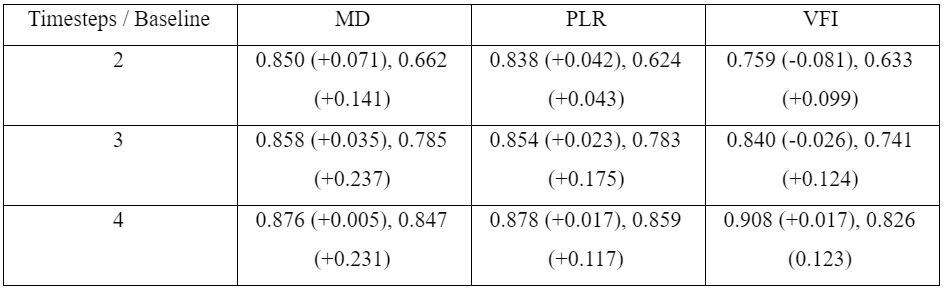
Table 3. Performance (accuracy, area under the ROC curve) of model trained on a given number of sequential visual fields and samples of clinical data (timesteps) with respect to ground truth from different traditional algorithms. The change in accuracy and area under the ROC curve from Table 2 is displayed in parentheses after each individual accuracy. MD = Mean Deviation, PLR = Pointwise Linear Regression, VFI = Visual Field Index.

ROC curves for each model are shown in Figures 4, 5, 6. Each pair of curves in each figure had identical train-test datasets to ensure comparability of results. 

In order to test the null hypothesis that there was no change in AUROC between a model that uses exclusively visual fields and a model supplemented with clinical data, a Z-test was used. Results from the Z-test for individual plots are in Table 4 and indicate statistical significance (p<0.01) for every plot, meaning that the diagnostic accuracy of a model supplemented by clinical data is better than a model that exclusively uses visual fields.

Table 4. Statistical comparison of the area under receiver operating characteristic curves with respect to different definitions of glaucoma progression for model 1 (visual field only) and model 2 (visual field and clinical data). MD = Mean Deviation, PLR = Pointwise Linear Regression, VFI = Visual Field Index.

In order to better understand the LTSM network after training, we determined the extent to which different points on the visual field contributed to the model’s decision making ability. Heatmaps for each model (MD slope, VFI slope, PLR) were created by subtracting the accuracy of the model after masking each individual point in the training dataset with the accuracy of the model trained on the original dataset.

Discussion

The primary aims of this study were to test the ability of a convolutional LSTM model to identify glaucoma progression and to determine whether supplementing visual fields with clinical data can improve performance. Evaluation against different baseline algorithms to define glaucoma worsening confirmed that the LSTM model was accurate in its predictions and could be trained to learn both global and local changes in visual fields. Training distinct networks on two data sources, specifically visual fields alone and visual fields supplemented with basic clinical data (cup to disc ratio, corneal thickness, and intraocular pressure) showed that the network trained on the combined data performed better.

A convolutional LSTM architecture performed well identifying glaucoma progression with AUROC values ranging from 0.82 to 0.90 when using both visual fields and clinical data as inputs. Although there is no agreed-upon objective definition of glaucoma progression, the proposed machine learning model is spatio-temporal by nature and shows it can learn both pointwise (as determined by PLR) and global (as determined by MD and VFI) trends. The presence of convolutional layers may allow it to extract spatial features that are not reflected in existing analyses. The combination of these factors makes the proposed ML architecture interpretable and an important step forward in finding a system that can synthesize for clinicians information relevant to glaucoma progression. Having an architecture that can incorporate multiple data sources is key to incorporating the same information used by clinicians which makes it more likely such a system will be used in clinical practice.

An important contribution of this work is the finding that supplementing visual fields with clinical data increased the performance of the model. The ROC curves of models with and without clinical data reveal that the sensitivity and specificity of the model using exclusively visual fields is significantly lower than those of a model supplemented by clinical data. The explanation for the high accuracy but low AUROC for the model trained exclusively on visual fields is class imbalance. The fact that the vast majority of eyes were determined to be stable (Table 1) makes it possible to achieve high accuracy simply by marking every eye as non-progressing.

One limitation of this study is the class imbalance and relatively small train/test sets. Either or both of these might affect the ability of the LTSM network to learn but the former is a feature of “real world” data and so may help us reflect performance in that setting. Though the ROC curves do imply that the proposed architecture had good specificity and sensitivity, there may have been other features the model learned that would hinder its ability to generalize. Another limitation is that only 4 visual fields were used to determine ground truth values from baseline algorithms. This was done in order to ensure sufficiently large train and test sets. However, it could mean that some of the ground truth values are inaccurate and thus that the network didn’t effectively learn “progression.” This could be addressed in future studies by combining data from multiple institutions in order to have larger data sets from which to learn. It may also be useful to include additional standards for identifying glaucoma progression such as physician assessment.

A logical follow up to this study would be to compare the ConvLSTM against other ML models that have been described. Similarly, it will be interesting to determine whether inclusion of data regarding optic nerve structure such as photographs and computerized imaging will make the ML network even better at predicting glaucoma progression. The clear challenge will be to define progression based not just on visual fields but also on optic nerve structural changes (i.e., do we require changes in either or both?) Finally, it will be interesting to see whether and how ML algorithms can incorporate other data from the EHR (other diagnoses, medications, procedures, etc.) and whether such data will meaningfully augment the data used so far.

While there is much interest in the latest revitalization of machine learning, which promises great potential for the future of glaucoma management, we should remember that the field itself is not new and that it generated similar excitement more than 20 years ago but then failed to transform medicine in a meaningful way. There is also increased awareness of the fact that these powerful algorithms are only able to learn from the examples we provide so a system that learns glaucoma at one institution may not generalize to another. We should therefore be cautious this time that we carefully evaluate and confirm that the algorithms we develop can indeed be used in settings with different patient populations so that we are not disappointed by the artificial intelligence future.

---

References

[1] Crabb DP, Garway-Heath DF. Intervals between visual field tests when monitoring the glaucomatous patient: wait-and-see approach. Invest Ophthalmol Vis Sci. 2012;53(6):2770. doi:10.1167/iovs.12-9476

[2] Heijl A, Bengtsson B, Chauhan BC, et al. A comparison of visual field progression criteria of 3 major glaucoma trials in early manifest glaucoma trial patients. Ophthalmology. 2008;115(9):1557-1565. doi:10.1016/j.ophtha.2008.02.005

[3] Giraud J-M, May F, Manet G, et al. Analysis of progression with gpa (Guided progression analysis) and mean deviation (Md) indexes of automated perimetry in ocular hypertension and glaucoma. Invest Ophthalmol Vis Sci. 2010;51(13):3997-3997.

[4] Katz J, Congdon N, Friedman DS. Methodological variations in estimating apparent progressive visual field loss in clinical trials of glaucoma treatment. Arch Ophthalmol. 1999;117(9):1137-1142. doi:10.1001/archopht.117.9.1137

[5] Aref AA, Budenz DL. Detecting visual field progression. Ophthalmology. 2017;124(12S):S51-S56. doi:10.1016/j.ophtha.2017.05.010

[6] Manassakorn A, Nouri-Mahdavi K, Koucheki B, Law SK, Caprioli J. Pointwise linear regression analysis for detection of visual field progression with absolute versus corrected threshold sensitivities. Invest Ophthalmol Vis Sci. 2006;47(7):2896-2903. doi:10.1167/iovs.05-1079

[7] Viswanathan A, Fitzke F, Hitchings R. Pointwise linear regression of glaucomatous visual fields. In: XIIIth International Perimetric Society Meeting. Gardone Riviera (BS), Italy: Kugler Publications; 1999:139-145. http://webeye.ophth.uiowa.edu/ips/cd/update98-99/139-146.pdf.

[8] Saeedi OJ, Elze T, D’Acunto L, et al. Agreement and predictors of discordance of 6 visual field progression algorithms. Ophthalmology. 2019;126(6):822-828. doi:10.1016/j.ophtha.2019.01.029

[9] Wang X, Wang F, Sontag D. Unsupervised learning of disease progression models. In: New York, USA: MIT; 2014. https://people.csail.mit.edu/dsontag/papers/WanSonWan_kdd14.pdf.

[10] Fisher CK, Smith AM, Walsh JR. Machine learning for comprehensive forecasting of Alzheimer’s Disease progression. Scientific Reports. 2019;9(1):1-14. doi:10.1038/s41598-019-49656-2

[11] Ting DSW, Cheung CY-L, Lim G, et al. Development and validation of a deep learning system for diabetic retinopathy and related eye diseases using retinal images from multiethnic populations with diabetes. JAMA. 2017;318(22):2211-2223. doi:10.1001/jama.2017.18152

[12] Caprioli J, Mock D, Bitrian E, et al. A method to measure and predict rates of regional visual field decay in glaucoma. Invest Ophthalmol Vis Sci. 2011;52(7):4765-4773. doi:10.1167/iovs.10-6414

[13] Yousefi S, Goldbaum MH, Balasubramanian M, et al. Glaucoma progression detection using structural retinal nerve fiber layer measurements and functional visual field points. IEEE Trans Biomed Eng. 2014;61(4):1143-1154. doi:10.1109/TBME.2013.2295605

[14] Wang M, Shen LQ, Pasquale LR, et al. An artificial intelligence approach to detect visual field progression in glaucoma based on spatial pattern analysis. Invest Ophthalmol Vis Sci. 2019;60(1):365-375. doi:10.1167/iovs.18-25568

[15] Lee J, Kim YK, Jeoung JW, Ha A, Kim YW, Park KH. Machine learning classifiers-based prediction of normal-tension glaucoma progression in young myopic patients. Jpn J Ophthalmol. 2020;64(1):68-76. doi:10.1007/s10384-019-00706-2

[16] Park K, Kim J, Lee J. Visual field prediction using recurrent neural network. Sci Rep. 2019;9. doi:10.1038/s41598-019-44852-6

[17] Murata H, Araie M, Asaoka R. A new approach to measure visual field progression in glaucoma patients using variational bayes linear regression. Invest Ophthalmol Vis Sci. 2014;55(12):8386-8392. doi:10.1167/iovs.14-14625

[18] Hogarty DT, Mackey DA, Hewitt AW. Current state and future prospects of artificial intelligence in ophthalmology: a review. Clin Experiment Ophthalmol. 2019;47(1):128-139. doi:10.1111/ceo.13381

[19] Kazemian P, Lavieri MS, Van Oyen MP, Andrews C, Stein JD. Personalized prediction of glaucoma progression under different target intraocular pressure levels using filtered forecasting methods. Ophthalmology. 2018;125(4):569-577. doi:10.1016/j.ophtha.2017.10.033

[20] Garway-Heath DF, Zhu H, Cheng Q, et al. Combining optical coherence tomography with visual field data to rapidly detect disease progression in glaucoma: a diagnostic accuracy study. Health Technol Assess. 2018;22(4):1-106. doi:10.3310/hta22040

[21] Cleeremans A, Servan-Schreiber D, McClelland JL. Finite state automata and simple recurrent networks. Neural Computation. 1989;1(3):372-381. doi:10.1162/neco.1989.1.3.372

[22] Hochreiter S, Schmidhuber J. Long short-term memory. Neural Computation. 1997;9(8):1735-1780. doi:10.1162/neco.1997.9.8.1735

[23] Shi X, Chen Z, Wang H, Yeung D-Y, Wong W, Woo W. Convolutional lstm network: a machine learning approach for precipitation nowcasting. arXiv:150604214 [cs]. September 2015. http://arxiv.org/abs/1506.04214. Accessed February 3, 2020.

[24] Cohen SL, Rosen AI, Tan X, Kingdom FAA. Improvement of the visual field index in clinical glaucoma care. Can J Ophthalmol. 2016;51(6):445-451. doi:10.1016/j.jcjo.2016.10.001

[25] Vesti E, Johnson CA, Chauhan BC. Comparison of different methods for detecting glaucomatous visual field progression. Invest Ophthalmol Vis Sci. 2003;44(9):3873-3879. doi:10.1167/iovs.02-1171

[26] Marín-Franch I, Swanson WH. The visualFields package: a tool for analysis and visualization of visual fields. J Vis. 2013;13(4). doi:10.1167/13.4.10

[27] Wen JC, Lee CS, Keane PA, et al. Forecasting future Humphrey Visual Fields using deep learning. PLoS One. 2019;14(4). doi:10.1371/journal.pone.0214875